#software #ai #llm #open-source
How to train a transformer based model, like LLaMA2, from scratch? Andrej Karpathy has open-sourced llama2.c project on GitHub. My learning process is “duplicate and rewrite”, which involves following the example but rewrite the code completely in my own coding style and language. I did the same and along the way I’ve learned something new. In this blog post, I’m going to break down the training code rewritten by myself, line by line, explain what and most importantly why.
Here is the source code repo of my rewritten code on Github: https://github.com/jimwang99/understanding-llm/tree/main/train
Model#
Architecture diagram: Understanding LLaMA2 Part 1 Model Architecture
Architecture hyper-parameters:
- $D$: dimension of embedding
- $N_l$: number of transformer layers
- $N_h$: number of heads
- $N_{kv}$: number of KV heads
- $V$: size of vocabulary
- $D_h$: hidden dimension of FFN layer
- $L_m$: max sequence length
- $L$: input sequence length
Tokenizer#
In Andrej’s example, Google’s sentencepiece is used, but more and more models use OpenAI’s tiktoken which has higher performance. So in my repo, I’ve prepared both types of tokenizers.
Prepare data#
TinyStories#
TinyStories is a dataset consists of short children stories only in English automatically generated by GPT. It is a perfect dataset for training mini transformer models.
- The story is simple and short, therefore you don’t need to have a large language model to understand and mimic its style. People has successfully trained 260K model, comparing to 7B or 70B sizes of general purpose foundation model.
- With smaller model in size, we can train it with normal GPUs. For example, I’ve trained it on my gaming station on a 3070 with only 8GB VRAM in only 10 hours.
- After training, the model can produce meaningful short stories with reasonable logic and grammar.
- It’s only English and has very limited vocabulary, so the
vocab_sizecan be small.
The original dataset is at https://huggingface.co/datasets/noanabeshima/TinyStoriesV2.
Using 4 different tokenizers, cl100k_base, r50k_base, sentencepiece_tok32k, sentencepiece_tok512, I’ve tokenized all the above entries and put them in https://huggingface.co/datasets/jimwang99/TinyStoriesV2-Tokenized.
Dataset#
In Andrej’s example, he created his own dataset serving class with random sharding support. In my repo, I’m using datasets from HuggingFace which support shuffle(), which has a much simpler implementation.
Loading dataset from HuggingFace#
self.dataset = datasets.load_dataset(
    "jimwang99/TinyStoriesV2-Tokenized", split=split
)- Dataset will be automatically downloaded if not already locally cached.
Iterator#
def __iter__(self) -> Iterator[Tuple[torch.Tensor, torch.Tensor]]:
    ...
    yield (input_tokens, output_targets)

def __next__(self):
    try:
        return next(self.iter)
    except RuntimeError as e:
        logger.warning(e)
        self.shuffle()
return next(self.iter)- Following Andrej’s example, I’ve also used iterator to return prepared tensors, so that we can concurrently run data preparation on CPU and forward/backward passes on GPU.
try ... except ...is used to captureStopIterationexception, which is converted toRuntimeErrorat runtime by Python interpreter, as in PEP479.
Construct a batch#
batch_seq_length = self.max_seq_length * self.batch_size

# get enough data from dataset
while len(buf) < batch_seq_length and idx < len(self.dataset):
    buf.extend(self.dataset[idx][self.tokenizer_name])
    idx += 1

# not enough data
if len(buf) < batch_seq_length and idx >= len(self.dataset):
raise StopIteration- Depend on how large a batch is and the max sequence length of each input token stream, tokens are concatenated into a buffer, which is later converted into tensor format.
- If the remaining data in the dataset it not enough for a batch, dataset is reshuffled automatically and restart from the very beginning.
JW: While serving data, we are trying to utilize all the available content from the dataset, each input stream of tokens does NOT naturally start from
BOS(begin of sequence) token. This randomness actually helps with generalization of trained model weights.
Training loop#
Initialization#
In the training loop, we need to create instances of model, tokenizer, datasets (for both training and validation), and optimizer.
Dataset splits#
Dataset are split into training and validation parts, usually 80% vs. 20%. Training data are used in forward/backward passes to calculate gradients and adjust the weights. Validation data are used every N # of iterations of training to calculate real losses, because those are the data that models never saw in its training loops.
dataset_eval = {}
dataset_eval["train"] = make_dataset(
    "train",
    tokenizer.name,
    max_seq_length=model.hparam.Lm,
    batch_size=config.batch_size,
    device=config.device,
)
dataset_eval["validation"] = make_dataset(
    "validation",
    tokenizer.name,
    max_seq_length=model.hparam.Lm,
    batch_size=config.batch_size,
    device=config.device,
)- In the dataset uploaded to
jimwang99/TinyStoriesV2-Tokenizedon HuggingFace, splits are already been made. Only need to specify their split names (as string) when creating dataset instances - In my repo, they are named with “train” and “validation” respectably
Optimizer#
We know that the training process of any ML models are:
- Initialize the model weights and biases.
- Run forward pass with training data and compare output with reference to calculate loss.
- Run backward pass using calculus chain-rules to calculate gradients of each weights and biases. Larger gradient means the corresponding weight or bias has larger impact on final loss.
- Adjust the weights and biases according to their gradient.
- Repeat 2~4 until we have good validation loss.
In step 4, there are many similar algorithms. Most famous one, which is used in all the deep-learning courses, is SGD (stochastic gradient descent), which is the simplest form of optimizer. On top of SGD, researchers have proposed many other algorithms, such as Adam (adaptive moment estimation, which added adaptive learning rate and momentum into the equation) and AdamW (which added weight decay regularization).
The goal of using different algorithms is to make training converge as quick as possible to a generalized local optimum, and reduce overall training time.
# optimizer
weight_decay: float = 0.01
adamw_beta1: float = 0.9
adamw_beta2: float = 0.999

def make_optimizer(
    model: torch.nn.Module,
    config: TrainingConfig,
) -> torch.optim.Optimizer:
    # use weight decay for parameters >= 2D
    decay_params = [
        p for _, p in model.named_parameters() if p.requires_grad and p.dim() >= 2
    ]
    nodecay_params = [
        p for _, p in model.named_parameters() if p.requires_grad and p.dim() < 2
    ]
    param_groups = [
        {"params": decay_params, "weight_decay": config.weight_decay},
        {"params": nodecay_params, "weight_decay": 0.0},
    ]
    return torch.optim.AdamW(
        param_groups,
        lr=config.max_learning_rate,
        betas=(config.adamw_beta1, config.adamw_beta2),
        fused=(config.device == "cuda"),
)- It’s very easy to create an AdamW optimizer in PyTorch.
- The only thing worth mentioning is
fusedparameter, which enables PyTorch to use C++ or CUDA version of AdamW, to achieve higher performance.
Learning rate#
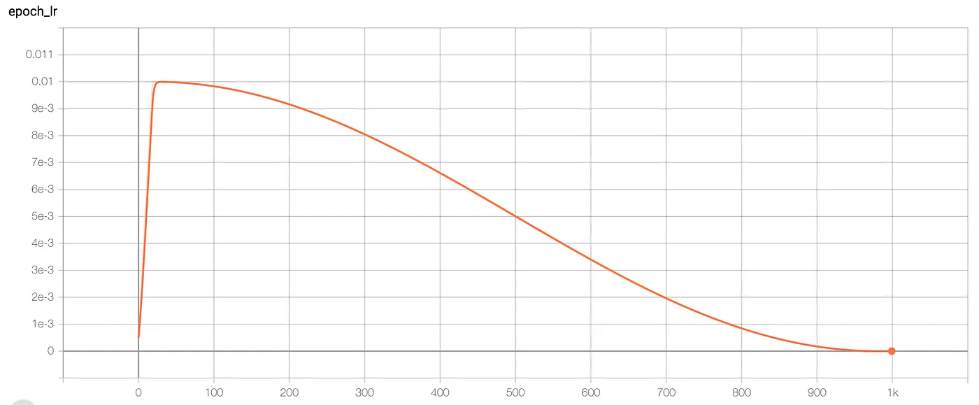
With optimizer, we need to give it guidance of how to adjust the weights, which is defined by learning rate. If we use a too small learning rate, the training process will take too long to converge; if we use a too large learning rate, the training process may not converge. I’ve followed Andrej’s example to use cosine learning rate decay, which has the following parameters:
is_learning_rate_decay: bool = True
num_warmup_iterations: int = 1000
max_decay_iterations: int = max_iterations
max_learning_rate: float = 1e-4
min_learning_rate: float = max_learning_rate * 0.1

def get_learning_rate(iter_idx: int, config: TrainingConfig) -> float:
    if config.is_learning_rate_decay is False:
        return config.max_learning_rate

    # warmup phase: linear increase
    if iter_idx < config.num_warmup_iterations:
        return config.max_learning_rate * iter_idx / float(config.num_warmup_iterations)
    # beyond phase: to min
    if iter_idx > config.max_decay_iterations:
        return config.min_learning_rate
    # decay phase: cosine decay down to min
    decay_ratio = (iter_idx - config.num_warmup_iterations) / (
        config.max_decay_iterations - config.num_warmup_iterations
    )
    assert 0.0 <= decay_ratio <= 1.0
    decay_coeff = 0.5 * (1.0 + math.cos(math.pi * decay_ratio))
    return config.min_learning_rate + decay_coeff * (
        config.max_learning_rate - config.min_learning_rate
)- It is separated into 3 phases
- First is warmup phase, starting from epoch 0, linearly increase to
max_learning_rate - Second is cosine decay phase, which slowly decrease the learning rate to
min_learning_ratefollowing a cosine wave - Third is beyond phase, where sticks to
min_learning_rate
Training iteration#
We entered the real training iteration, which consists of loops of forward, backward and parameter update. Each iteration we run it with a batch of input data.
Batch size#
To maximize the utilization of GPU, you need to carefully select the right batch_size number, so that it won’t exceed its memory capacity. You can use nvtop to exam the memory usage of your GPU.
Gradient accumulation#
If you are not using state-of-the-art GPUs, like H100 in 2024, the batch size won’t be large enough to make the training process generalized. Therefore, we can accumulate the gradients by running multiple batches, then step the weights and biases.
# ----------------------------------------------------------------------
# forward / backward
# ----------------------------------------------------------------------
input_tokens, output_targets = next(dataset)
for _ in range(config.gradient_accumulation_steps):
    # foward
    output_logits = model.forward(input_tokens)

    # calculate loss
    loss = get_loss(output_logits, output_targets)
    loss = loss / config.gradient_accumulation_steps

    # backward
    loss.backward()

    # prefetch next batch of data
    input_tokens, output_targets = next(dataset)
# ----------------------------------------------------------------------
# step advance optimizer
# ----------------------------------------------------------------------
if config.gradient_clip != 0.0:
    torch.nn.utils.clip_grad_norm_(
        model.parameters(), max_norm=config.gradient_clip
    )
optimizer.step()
optimizer.zero_grad()- In above code example,
gradient_accumulation_steps# of forward/backward passes are run before we step the optimizer. - In above code, you probably noticed
gradient_clipparameter. We use gradient clip to prevent gradients from becoming too large, to stabilize the training process. - After weights and biases are updated, gradients are zeroed for the next batch of forward and backward passes.
Evaluation#
Evaluation step is used to monitor the loss of the model using a different set of data that’s not in the training dataset. It’s for monitoring the progress of the training, and can be used to save checkpoints as well.
Getting evaluation set loss
loss = {}
model.eval()
with torch.inference_mode():
    for split in dataset_eval.keys():
        losses = torch.zeros(config.eval_iterations)
        for idx, (input_tokens, output_targets) in enumerate(
            dataset_eval[split]
        ):
            if idx >= config.eval_iterations:
                break
            output_logits = model.forward(input_tokens)
            losses[idx] = get_loss(output_logits, output_targets)
        loss[split] = losses.mean()
    for split in dataset_eval.keys():
        logger.debug(f"dataset={split} loss={loss[split]}")
model.train()
Save checkpoints
# save if loss is smaller than minimum
if loss["validation"] < min_loss:
    logger.debug(f"min_loss: {min_loss:.4f} -> {loss['validation']:.4f}")
    min_loss = loss["validation"]

    if iter_idx > 0:
        logger.debug("Saving checkpoint")
        checkpoint = {
            "model": model.state_dict(),
            "optimizer": optimizer.state_dict(),
            "iter_idx": iter_idx,
            "min_loss": min_loss,
            "config": config,
        }
        torch.save(checkpoint, f"checkpoint.{config.name}.pt")

elapsed_time_hour = (time.time() - start_time) / 3600.0
logger.info(
    f"<SUMMARY> {iter_idx} | loss {min_loss:.4f} | lr {lr:e} | elapsed {elapsed_time_hour:.2f}hrs"
)
pmon.loop()Summary#
That’s it.
You can clone the repo, adjust the batch size and kick off a training on your GPU right away.